Foundations of Causal Inference: Observational Studies

Lecture 23

Author

Affiliation

Josh Lim

Duke University
STA 199 Summer 2026: Session 2
Adapted from slides by Mine Çetinkaya-Rundel, Katie Solarz & John Zito

Revisiting confounding

What changes without randomization?

• In an observational study, the researcher does not assign treatment — subjects choose (or are assigned by nature)

• This means \(Z\) is not independent of \(X\): people who receive treatment differ systematically from those who do not

• The backdoor path \(X \to Z \to Y\) is open, and the naive difference in means conflates the treatment effect with confounding

• \(E[\bar{Y}_{\text{treated}} - \bar{Y}_{\text{control}}] \neq \tau\)

The core problem

• Students who seek tutoring tend to be those who are struggling — lower prior GPA

• If we compare exam scores, tutored students may still score lower even if tutoring helps

• Conversely, employees who get promoted might be higher performers to begin with — making the promotion look more effective than it is

• We need a way to make treated and control groups comparable on \(X\) without running an experiment

Matching on covariates

The idea of matching

• For each treated unit, find one (or more) control units that look similar on \(X\)

• Compare outcomes within matched pairs — differences now reflect treatment, not confounding

• We are trying to mimic a randomized experiment by constructing comparable groups from observational data

Formally

• The key assumption: conditional ignorability

\[Y(0), Y(1) \perp Z \mid X\]

• Given covariates \(X\), treatment assignment is “as good as random”

• This is also called no unmeasured confounders — a strong, untestable assumption

• If it holds, matching on \(X\) recovers the causal effect

An example with matching

The data

We use the LaLonde dataset: a study of a 1970s job training program. Participants were not randomly assigned.

data("lalonde", package = "MatchIt")
glimpse(lalonde)

Rows: 614
Columns: 9
$ treat    <int> 1, 1, 1, 1, 1, 1, 1, 1, 1, 1, 1, 1, 1, 1, 1, 1, 1, …
$ age      <int> 37, 22, 30, 27, 33, 22, 23, 32, 22, 33, 19, 21, 18,…
$ educ     <int> 11, 9, 12, 11, 8, 9, 12, 11, 16, 12, 9, 13, 8, 10, …
$ race     <fct> black, hispan, black, black, black, black, black, b…
$ married  <int> 1, 0, 0, 0, 0, 0, 0, 0, 0, 1, 0, 0, 0, 1, 0, 0, 0, …
$ nodegree <int> 1, 1, 0, 1, 1, 1, 0, 1, 0, 0, 1, 0, 1, 1, 1, 1, 0, …
$ re74     <dbl> 0, 0, 0, 0, 0, 0, 0, 0, 0, 0, 0, 0, 0, 0, 0, 0, 0, …
$ re75     <dbl> 0, 0, 0, 0, 0, 0, 0, 0, 0, 0, 0, 0, 0, 0, 0, 0, 0, …
$ re78     <dbl> 9930.0460, 3595.8940, 24909.4500, 7506.1460, 289.78…

• treat: 1 = job training, 0 = no training
• re78: earnings in 1978 (outcome \(Y\))
• age, educ, re74, re75, etc.: covariates \(X\)

Naive estimate (no matching)

lalonde |>
  group_by(treat) |>
  summarise(mean_earnings = mean(re78))

# A tibble: 2 × 2
  treat mean_earnings
  <int>         <dbl>
1     0         6984.
2     1         6349.

• The naive difference suggests training increases earnings

• But treated and control groups may differ on pre-treatment characteristics — we can’t trust this yet

Check for imbalance

lalonde |>
  group_by(treat) |>
  summarise(mean_age  = mean(age),
            mean_educ = mean(educ),
            mean_re74 = mean(re74),
            mean_re75 = mean(re75))

# A tibble: 2 × 5
  treat mean_age mean_educ mean_re74 mean_re75
  <int>    <dbl>     <dbl>     <dbl>     <dbl>
1     0     28.0      10.2     5619.     2466.
2     1     25.8      10.3     2096.     1532.

• Treated individuals have lower prior earnings (re74, re75) — confounding is present

• We need to adjust for this before drawing causal conclusions

Nearest-neighbor matching

m_out <- matchit(treat ~ age + educ + re74 + re75,
                 data   = lalonde,
                 method = "nearest")
summary(m_out, un = FALSE)

Call:
matchit(formula = treat ~ age + educ + re74 + re75, data = lalonde, 
    method = "nearest")

Summary of Balance for Matched Data:
         Means Treated Means Control Std. Mean Diff. Var. Ratio
distance        0.3536        0.3523          0.0141     1.0160
age            25.8162       25.2811          0.0748     0.4690
educ           10.3459       10.4486         -0.0511     0.6392
re74         2095.5737     2137.7507         -0.0086     1.2576
re75         1532.0553     1385.2355          0.0456     1.7520
         eCDF Mean eCDF Max Std. Pair Dist.
distance    0.0088   0.0757          0.0179
age         0.0801   0.2486          1.4014
educ        0.0208   0.0973          1.0673
re74        0.0365   0.2541          0.1778
re75        0.0379   0.1946          0.6412

Sample Sizes:
          Control Treated
All           429     185
Matched       185     185
Unmatched     244       0
Discarded       0       0

Estimate on matched data

m_data <- match.data(m_out)

lm(re78 ~ treat, data = m_data, weights = weights) |> tidy()

# A tibble: 2 × 5
  term        estimate std.error statistic  p.value
  <chr>          <dbl>     <dbl>     <dbl>    <dbl>
1 (Intercept)    5988.      533.    11.2   2.38e-25
2 treat           362.      754.     0.479 6.32e- 1

• After matching, the estimate is our best causal estimate under the ignorability assumption

• Compare this to the naive estimate — confounding matters!

The high-dimension problem

Curse of dimensionality

• Matching works well when \(X\) has only a few variables

• With many covariates, it becomes nearly impossible to find good matches — the space is too sparse

• Example: match exactly on age (35), education (12 years), prior earnings ($8,000), race, marital status…

• The probability of finding a near-identical control unit vanishes as the dimension of \(X\) grows

We need a smarter approach

• Instead of matching on the full \(X\) vector, collapse it to a single number

• The propensity score:

\[e(X) = P(Z = 1 \mid X)\]

• The probability of receiving treatment, given covariates

• Rosenbaum & Rubin (1983): if \(Y(0), Y(1) \perp Z \mid X\), then also \(Y(0), Y(1) \perp Z \mid e(X)\)

• Matching on this one number is sufficient!

Propensity score matching

Estimating the propensity score

We estimate \(e(X)\) via logistic regression:

\[\log\frac{P(Z=1 \mid X)}{1 - P(Z=1 \mid X)} = \beta_0 + \beta_1 X_1 + \cdots + \beta_p X_p\]

• Fit logistic regression of \(Z\) on \(X\)

• Predicted probabilities \(\hat{e}(X_i)\) are the estimated propensity scores

• Match treated and control units with similar \(\hat{e}(X)\) values

The workflow

1. Fit a logistic regression model: \(Z \sim X_1 + \cdots + X_p\)
2. Extract predicted probabilities as propensity scores
3. Match treated to control units with similar scores
4. Check balance on \(X\) in the matched sample
5. Estimate the treatment effect on the matched data

Propensity score matching example

Step 1 & 2: fit model, get scores

ps_model <- glm(treat ~ age + educ + re74 + re75,
                data   = lalonde,
                family = binomial)

lalonde <- lalonde |>
  mutate(ps = predict(ps_model, type = "response"))

lalonde |>
  group_by(treat) |>
  summarise(mean_ps = mean(ps), sd_ps = sd(ps))

# A tibble: 2 × 3
  treat mean_ps  sd_ps
  <int>   <dbl>  <dbl>
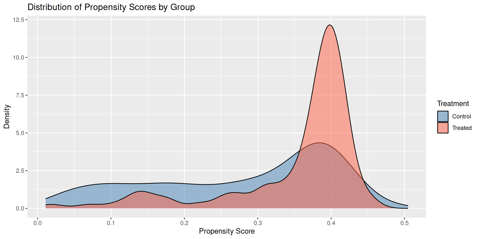
1     0   0.279 0.126 
2     1   0.354 0.0901

Visualize the scores

Step 3 & 4: match and check balance

ps_match <- matchit(treat ~ age + educ + re74 + re75,
                    data     = lalonde,
                    method   = "nearest",
                    distance = "glm")

summary(ps_match, un = FALSE)

Call:
matchit(formula = treat ~ age + educ + re74 + re75, data = lalonde, 
    method = "nearest", distance = "glm")

Summary of Balance for Matched Data:
         Means Treated Means Control Std. Mean Diff. Var. Ratio
distance        0.3536        0.3523          0.0141     1.0160
age            25.8162       25.2811          0.0748     0.4690
educ           10.3459       10.4486         -0.0511     0.6392
re74         2095.5737     2137.7507         -0.0086     1.2576
re75         1532.0553     1385.2355          0.0456     1.7520
         eCDF Mean eCDF Max Std. Pair Dist.
distance    0.0088   0.0757          0.0179
age         0.0801   0.2486          1.4014
educ        0.0208   0.0973          1.0673
re74        0.0365   0.2541          0.1778
re75        0.0379   0.1946          0.6412

Sample Sizes:
          Control Treated
All           429     185
Matched       185     185
Unmatched     244       0
Discarded       0       0

Step 5: estimate the effect

ps_data <- match.data(ps_match)

lm(re78 ~ treat, data = ps_data, weights = weights) |> tidy()

# A tibble: 2 × 5
  term        estimate std.error statistic  p.value
  <chr>          <dbl>     <dbl>     <dbl>    <dbl>
1 (Intercept)    5988.      533.    11.2   2.38e-25
2 treat           362.      754.     0.479 6.32e- 1

• After propensity score matching, we have a valid causal estimate (under ignorability)

• The propensity score approach scales to many covariates, unlike direct matching

• Always check balance after matching — if it’s poor, consider a different model for the propensity score

Key takeaways

• Observational studies require careful adjustment for confounders \(X\)

• Matching reconstructs comparability between treated and control groups

• Direct matching works with few covariates; propensity score matching scales to high dimensions

• All methods require no unmeasured confounders — this assumption cannot be tested from data alone

• Sensitivity analyses can assess how robust conclusions are to potential unmeasured confounding