Linear Regression Diagnostics

Lecture 16

Author
Affiliation

Josh Lim

Duke University
STA 199 Summer 2026: Session 2
Adapted from slides by Mine Çetinkaya-Rundel, Katie Solarz & John Zito

Published

July 24, 2026

Commentary on Projects

Milestone 3 primer

Today’s Topics

  • Finish AE-14

  • Model assumptions

  • Model diagnostics

AE-14

Quick Notes

  • When interpreting intercepts and slopes in the context of any linear regression modeling, your interpretation should include both of the following phrases: “we expect” (or functionally similar) AND “on average”

  • When you’ve fit a multiple linear regression model (i.e., > 1 predictor), your slope interpretations must also include the following: “all else equal” (or functionally similar)

  • I know it’s prescriptive and somewhat repetitive, but for your own sanity (& mine <3), please please include these statements in every interpretation you provide

Model Assumptions

But first, a quick game

  • 10-carat old mine brilliant-cut diamond
  • 58 facets
  • Est. at $550K - $1M

  • 5-carat antique cushion-cut diamond
  • $280,000 price tag

  • Est. 30-40-carat high color center diamond
  • 1-carat oval side stones
  • Est. value upwards of $3M

The 4 Cs

When evaluating a diamond, jewelers typically focus on four key characteristics known as the 4 Cs:

  • Carat — How big is it?
  • Cut — How much does it sparkle?
  • Clarity — How flawless is it?
  • Color — How colorless is it?

The 4 Cs are the primary factors that determine a diamond’s value.

Today’s Data

set.seed(847)
diamonds <- read_csv("data/diamonds.csv") |>
  rename(length_mm = x, width_mm = y) |>
  select(price, carat, cut, color, clarity, length_mm, width_mm) |>
  mutate(color = factor(color),
         cut = fct_relevel(cut, c("Ideal", "Premium", "Very Good", "Good", "Fair")),
         clarity = factor(clarity)) |>
  mutate(clarity = fct_collapse(clarity,
    "IF" = "IF",
    "VVS" = c("VVS1", "VVS2"),
    "VS" = c("VS1", "VS2"),
    "SI" = c("SI1", "SI2"),
    "I" = "I1")) |>
  mutate(clarity = fct_relevel(clarity, c("IF", "VVS", "VS", "SI", "I"))) |>
  filter(carat <= 3.0) |>
  sample_n(5000)

glimpse(diamonds)
Rows: 5,000
Columns: 7
$ price     <dbl> 3867, 12048, 878, 4325, 401, 5504, 1767, 4704, 112…
$ carat     <dbl> 0.90, 2.01, 0.41, 0.68, 0.30, 1.19, 0.63, 1.02, 0.…
$ cut       <fct> Ideal, Ideal, Very Good, Ideal, Ideal, Ideal, Good…
$ color     <fct> I, J, F, D, E, D, H, G, F, H, F, G, H, I, I, F, F,…
$ clarity   <fct> VS, SI, SI, VVS, SI, SI, VS, SI, SI, VS, VS, VVS, …
$ length_mm <dbl> 6.13, 8.08, 4.73, 5.66, 4.33, 6.91, 5.47, 6.36, 5.…
$ width_mm  <dbl> 6.18, 8.03, 4.69, 5.69, 4.35, 6.89, 5.56, 6.40, 5.…


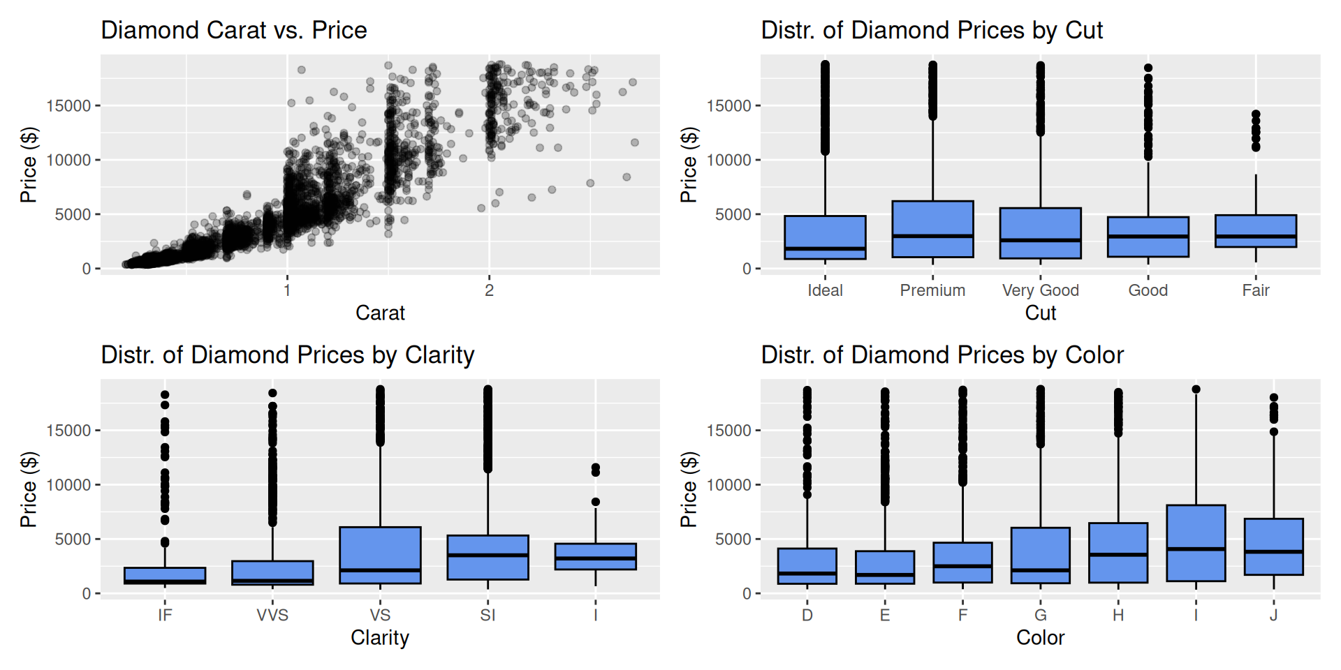
Bivariate EDA

Let’s start with SLR

Fitted Model:

diamond_fit_ct <- linear_reg() |>
  fit(price ~ carat, data = diamonds)

tidy(diamond_fit_ct)
# A tibble: 2 × 5
  term        estimate std.error statistic p.value
  <chr>          <dbl>     <dbl>     <dbl>   <dbl>
1 (Intercept)   -2361.      41.9     -56.3       0
2 carat          7916.      45.2     175.        0

Using statistical notation…

\[ \widehat{\text{price}} = -2360.588 + 7916.132 \times \text{carat} \]

How would you interpret the intercept in the context of these data–is it meaningful? What about the slope?

The 4 Assumptions (of linear regression modeling)

Just as a diamond’s value depends on its 4 Cs, the reliability of a linear regression model depends on its 4 core assumptions

\[ Y|X_1, \ldots, X_p \sim N(\beta_0 + \beta_1X_1 + \dots + \beta_pX_p, \sigma_\epsilon^2) \]

The above is what we implicitly assume to be true when we preform standard regression modeling; this is a fancy expression (take STA 240, 210, or 221 to learn more!) that basically encapsulates the following:

  1. Independence: The errors (residuals) are independent from one another.

  2. Linearity: There is a linear relationship between the response and predictor variables.

  3. Equal variance: The variability about the least squares line is equal for all combinations of predictors.

  4. Normality: The distribution of the errors (residuals) is approximately normal.

1. Independence

Recall our population model for the \(i^{th}\) observation \[ y_i = \beta_0 + \beta_1 x_{i1} + \beta_2 x_{i2} + ...+ \beta_p x_{ip} +\epsilon_i \]

Independence: The errors \(\epsilon_i\) are independent of one another. Specifically, this also implies that the outcomes \(y_i\) are independent (don’t worry about why).

How might the independence assumption be violated?

Remember this crap?

The Treatment of Lead-Exposed Children (TLC) Trial was a placebo-controlled, randomized clinical trial designed to evaluate whether treatment with succimer, an oral chelating agent used to remove lead from the body, could reduce blood lead levels in young children with moderate lead exposure. The study enrolled children aged 12–33 months with blood lead levels between 20 and 44 micrograms per deciliter (µg/dL) and randomly assigned them to receive either succimer or a placebo. Blood lead levels were measured repeatedly over time to assess the effectiveness of the treatment.

tlc_raw <- read_csv("data/tlc_raw.csv")

tlc_long <- tlc_raw |>
  pivot_longer(
    cols = -c(id, group),
    names_to = "week",
    names_prefix = "lead_w",
    names_transform = as.numeric,
    values_to = "lead_lvl"
  )

glimpse(tlc_long)
Rows: 400
Columns: 4
$ id       <dbl> 1, 1, 1, 1, 2, 2, 2, 2, 3, 3, 3, 3, 4, 4, 4, 4, 5, …
$ group    <chr> "P", "P", "P", "P", "A", "A", "A", "A", "A", "A", "…
$ week     <dbl> 0, 1, 4, 6, 0, 1, 4, 6, 0, 1, 4, 6, 0, 1, 4, 6, 0, …
$ lead_lvl <dbl> 30.8, 26.9, 25.8, 23.8, 26.5, 14.8, 19.5, 21.0, 25.…

What might be problematic here if I fit a model predicting lead_lvl from both group and week using these data?

2. Linearity

Back to our population model… \[ y = \beta_0 + \beta_1 x_{1} + \beta_2 x_{2} + ...+ \beta_p x_{p} +\epsilon \]

Linearity:The regression model is linear in the parameters. Specifically, this is a linearity assumption on the parameters (i.e., the \(\beta\) terms), NOT the predictors themselves (i.e., the observed x terms).

So this is fine…

\[ y = \beta_0 + \beta_1 x_{1} + \beta_2 x_{2}^2 + ...+ \beta_p x_{p}^p +\epsilon \]

… but this is not.

\[ y = \beta_0 + \frac{\beta_1x_1}{\beta_2 + \beta_3(x_1+1)} +...+ \beta_p x_{p} +\epsilon \]

3. Equal variance

\[ y_i = \beta_0 + \beta_1 x_{i1} + \beta_2 x_{i2} + ...+ \beta_p x_{ip} +\epsilon_i \] \[ \epsilon_i \overset{\text{i.i.d}}\sim N(0, \sigma^2) \] Equal variance: The variance of the errors is constant (per the notation above, this variance is some constant represented by \(\sigma^2\)) regardless of what the predictor values are. Specifically, this also implies that the variance of the errors is independent of the predictors.

This may sound a bit abstract, and you don’t need to fret over any of the fancy notation. For the purposes of this course, we’ll just show you how to check whether or not this assumption is reasonably satisfied.

4. Normality

Again, in fancy notation:

\[ \epsilon_i \overset{\text{i.i.d}}\sim N(0, \sigma^2) \]

Normality: The errors follow a normal (bell-shaped) distribution centered at zero.

Model diagnostics

So, how do we check?

Independence

  • We usually have to think through this one, unfortunately. In some situations there might be some plots that will specifically give us an indication that independence is violated, but it’s best practice to think about the data generating mechanism and how the observations actually came about. Understanding experimental design is especially helpful here.

  • In a randomized experiment, independence across subjects is often a reasonable assumption because the randomization process helps prevent observations from systematically influencing one another (e.g., we can assume that one child’s blood lead levels do not indluence a different child’s blood lead levels in the TLC trial).

  • In observational studies, however, we need to think more carefully about whether observations may be related through time, location, shared environments, repeated measurements, or other sources of dependence.

Residual plots help with the rest!

First, get the residuals and “fitted” (predicted) values for your original data with augment():

diamonds_aug <- augment(diamond_fit_ct, diamonds)

glimpse(diamonds_aug)
Rows: 5,000
Columns: 9
$ .pred     <dbl> 4763.93087, 13550.83688, 885.02641, 3022.38193, 14…
$ .resid    <dbl> -896.930869, -1502.836879, -7.026414, 1302.618070,…
$ price     <dbl> 3867, 12048, 878, 4325, 401, 5504, 1767, 4704, 112…
$ carat     <dbl> 0.90, 2.01, 0.41, 0.68, 0.30, 1.19, 0.63, 1.02, 0.…
$ cut       <fct> Ideal, Ideal, Very Good, Ideal, Ideal, Ideal, Good…
$ color     <fct> I, J, F, D, E, D, H, G, F, H, F, G, H, I, I, F, F,…
$ clarity   <fct> VS, SI, SI, VVS, SI, SI, VS, SI, SI, VS, VS, VVS, …
$ length_mm <dbl> 6.13, 8.08, 4.73, 5.66, 4.33, 6.91, 5.47, 6.36, 5.…
$ width_mm  <dbl> 6.18, 8.03, 4.69, 5.69, 4.35, 6.89, 5.56, 6.40, 5.…

Residual plots help with the rest!

Then, explore & assess!

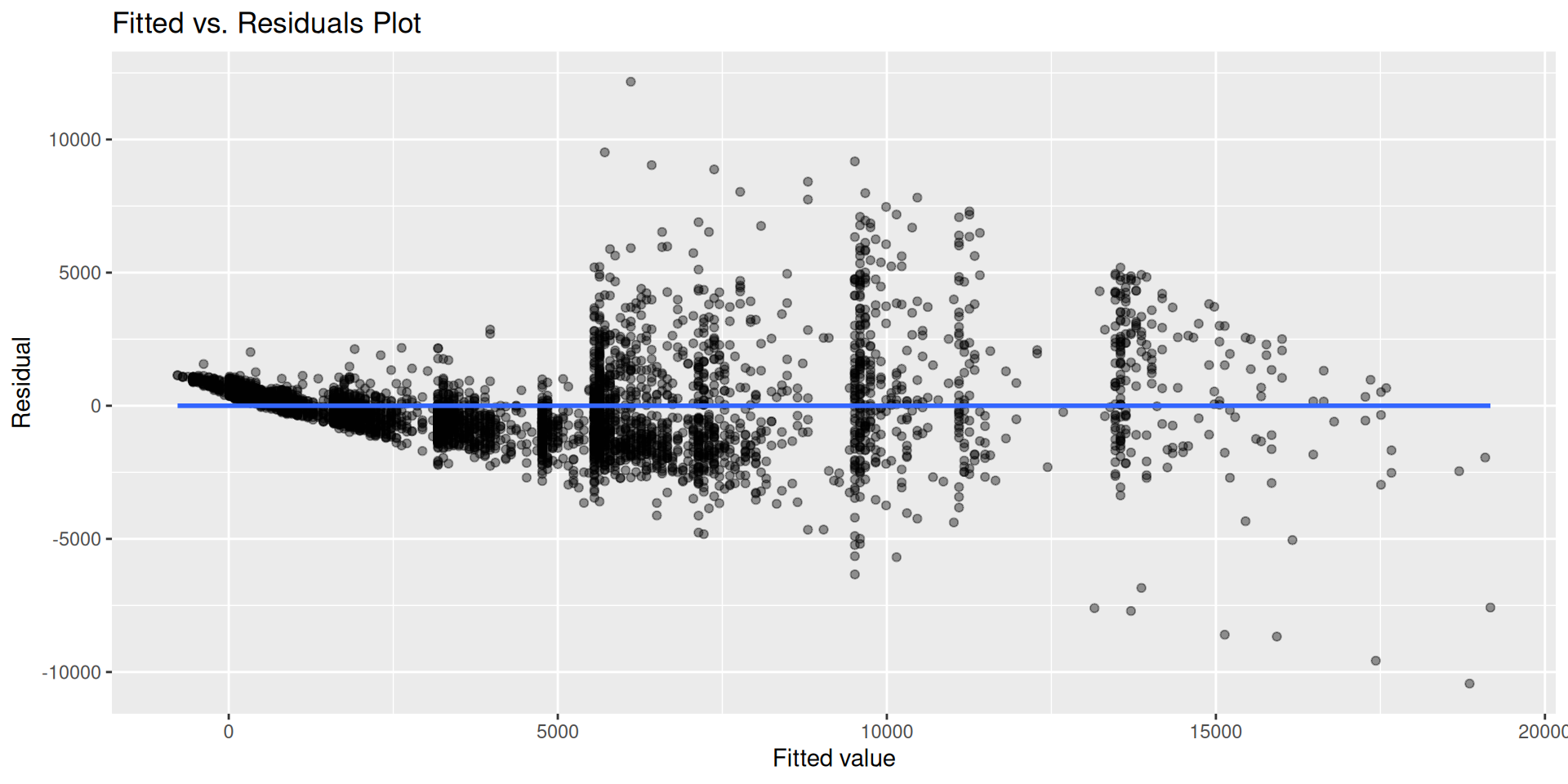
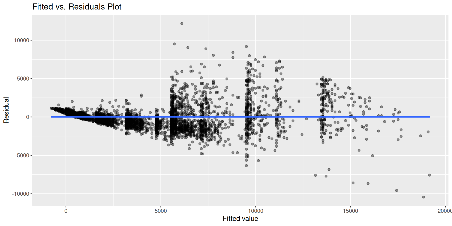
First, a “Fitted vs. Residuals” plot:

ggplot(diamonds_aug, aes(x = .pred, y = .resid)) +
  geom_point(alpha = 0.4) +
  geom_smooth(method = "lm", se = FALSE) +
  labs(x = "Fitted value",
       y = "Residual",
       title = "Fitted vs. Residuals Plot")

What are we looking for?

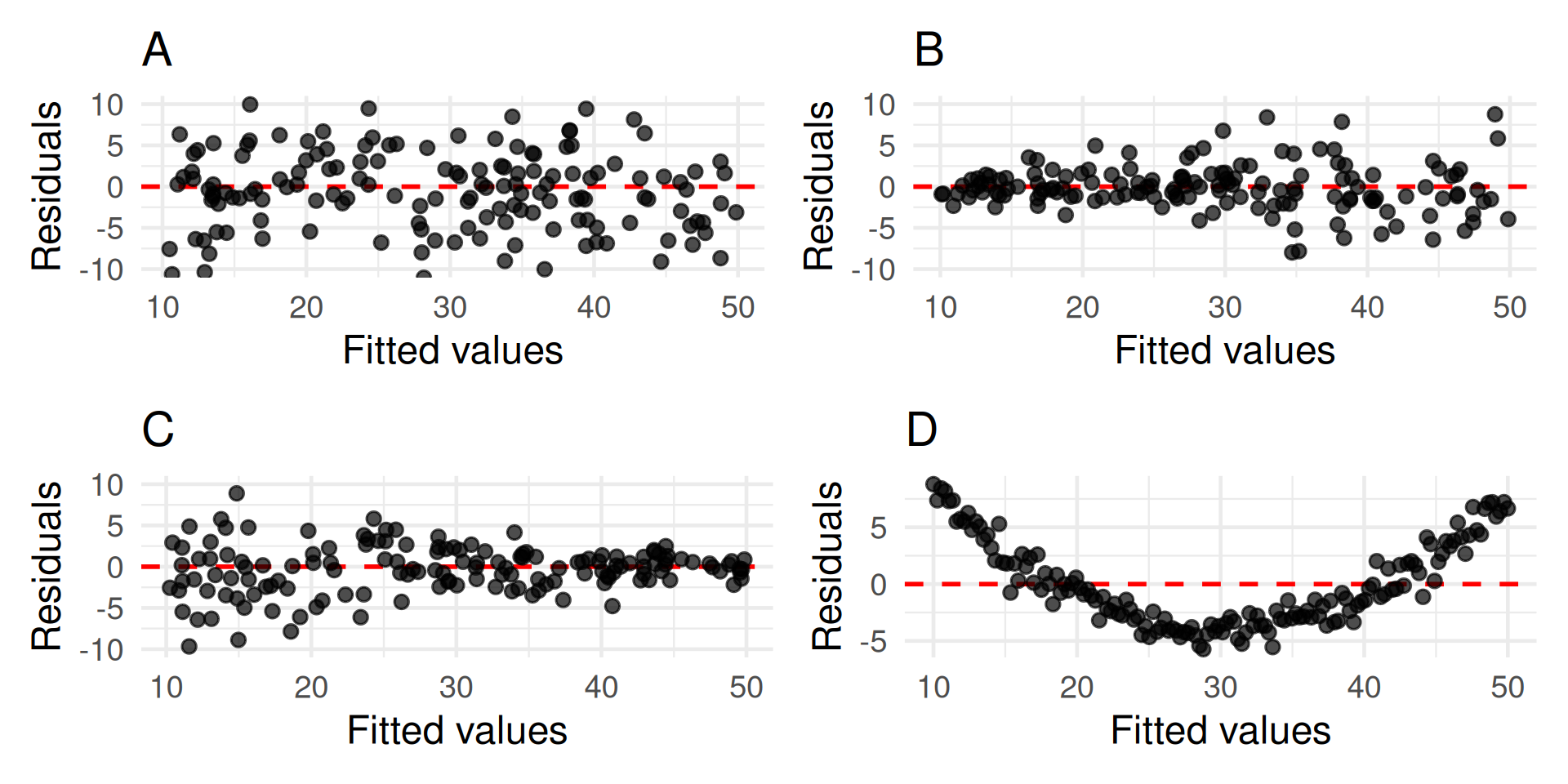
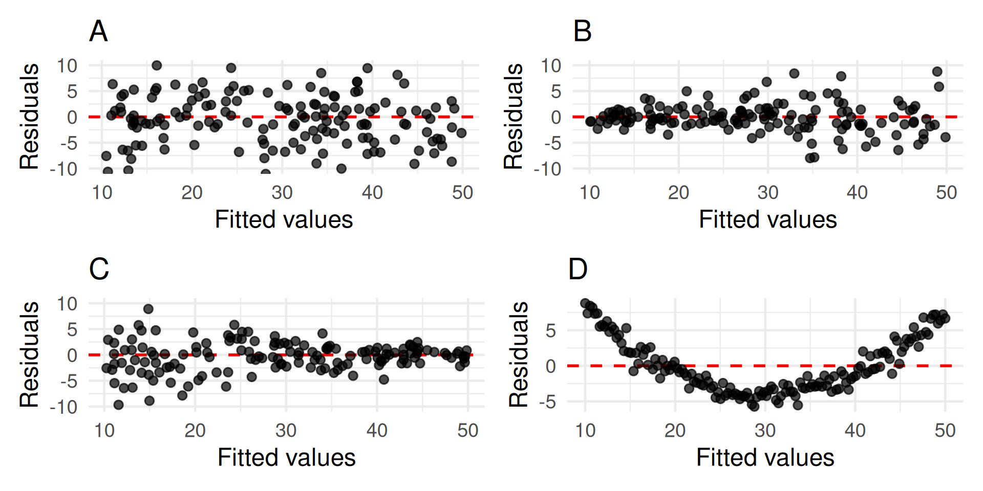
  • Linearity: If linearity is satisfied, we would expect to find no discernible pattern (i.e., points randomly scattered around the horizontal axis \(\text{y} = 0\)) in the fitted vs. residuals plot

  • Equal variance: If equal variance is satisfied, we would expect to see “evenly-spaced” dots (in the vertical sense) along the y-axis, regardless of what the predicted values are.

What are we looking for?

  • In the above, plot A is an example of a “good” fitted vs. residuals plot that supports both the linearity and equal variance assumptions (homoskedastic data)

  • Plot B shows that the residual variance (vertical spread) increases as the fitted values increase; plot C shows the residual variance decreasing as the fitted values increase

    • Both of these plots suggest that the underlying model violates the assumption of constant / equal error variance (heteroskedastic data)
  • Plot D shows a curved pattern, which indicates that the wrong type of model was used (i.e., linearity assumption is violated)

Back to the diamonds!

Based on the fitted vs. residuals plot below, what do you think of the linearity and constant variance assumptions underlying our simple linear regression model predicting diamond price from carat?

Distribution of residuals

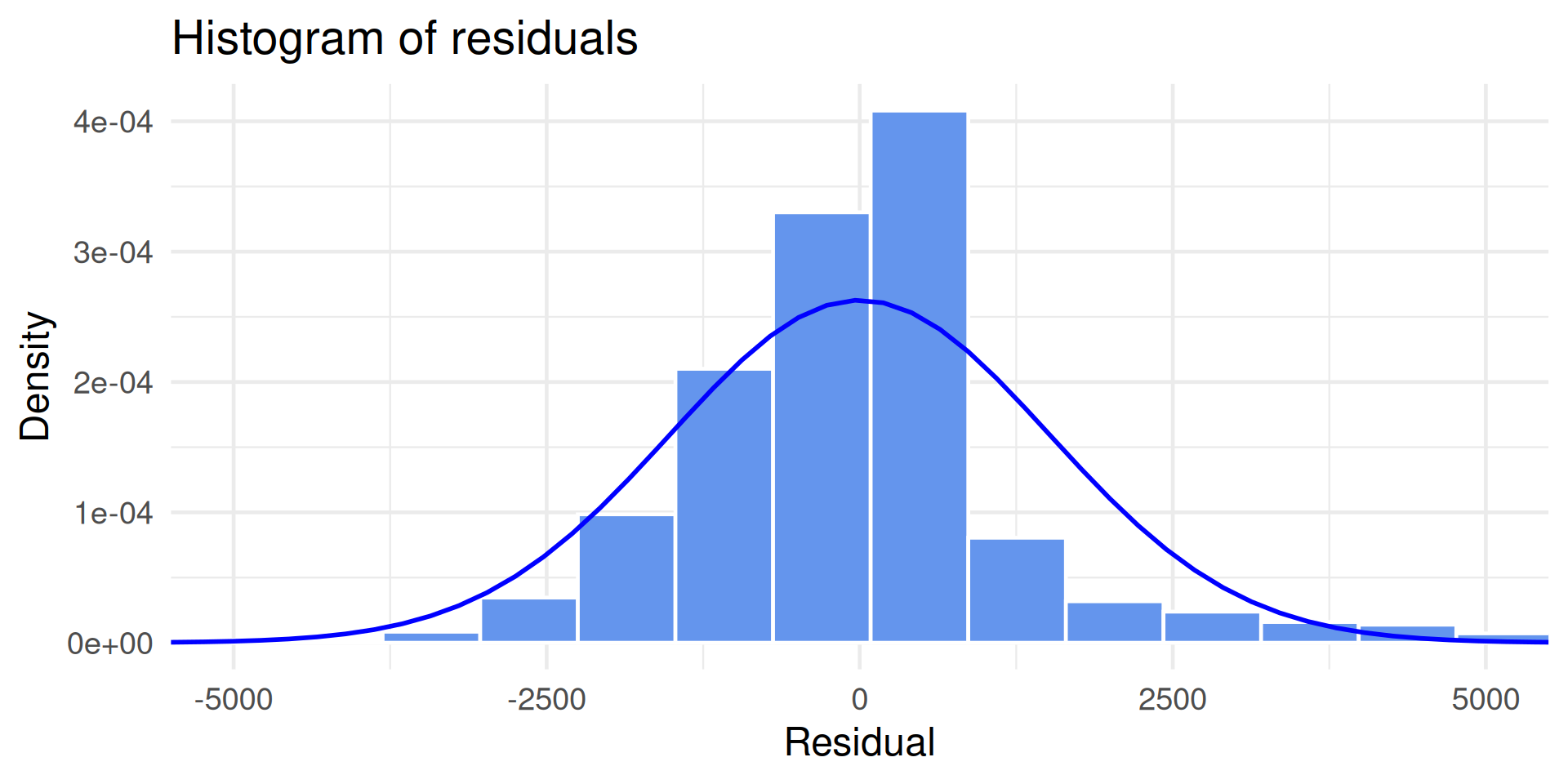
  • Next, we can take a look at a histogram of the residuals to get an overall feel for the distribution of them

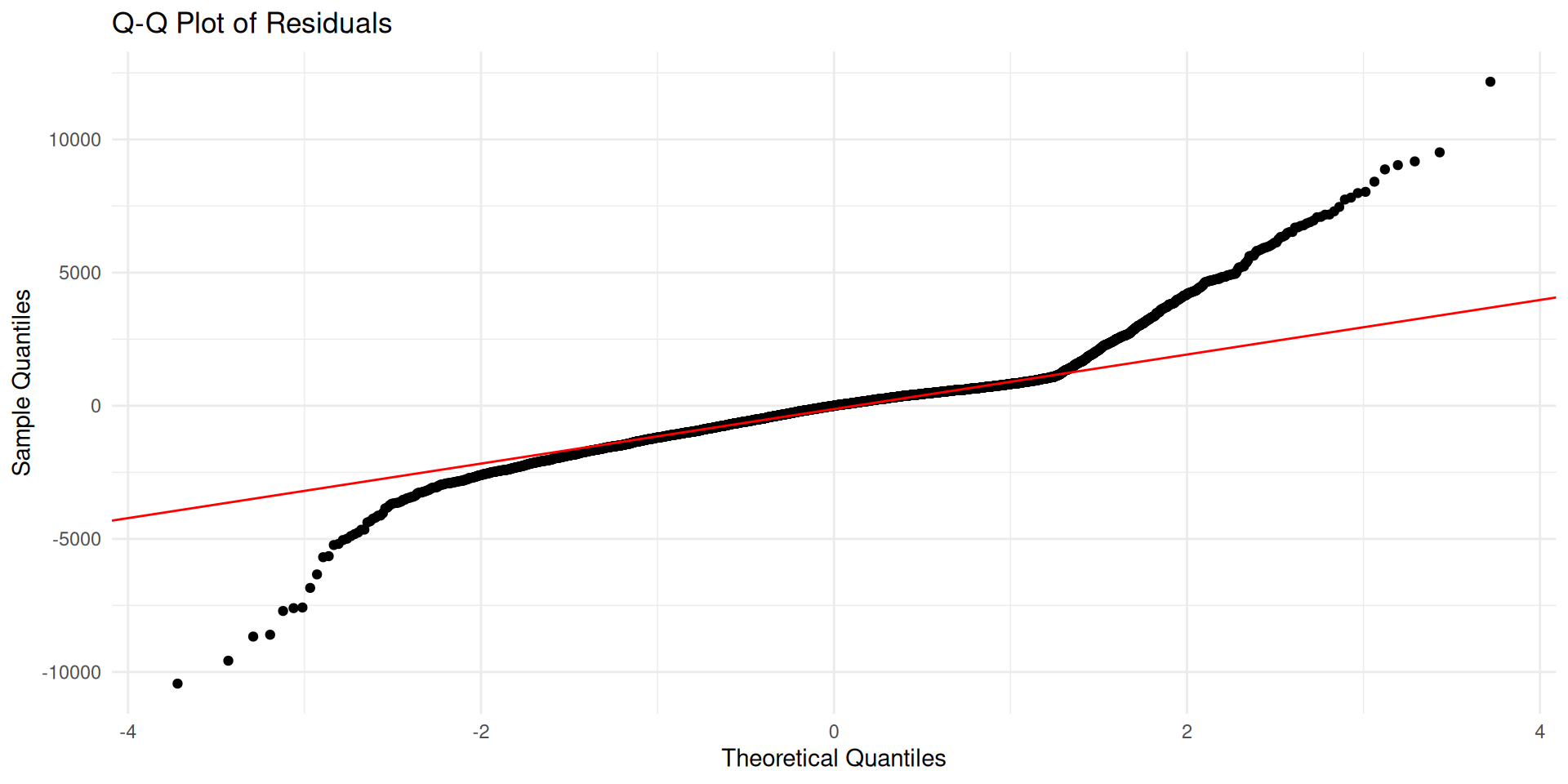
  • Alternatively, we can use a quantile-quantile plot (Q-Q plot) to get a more accurate picture

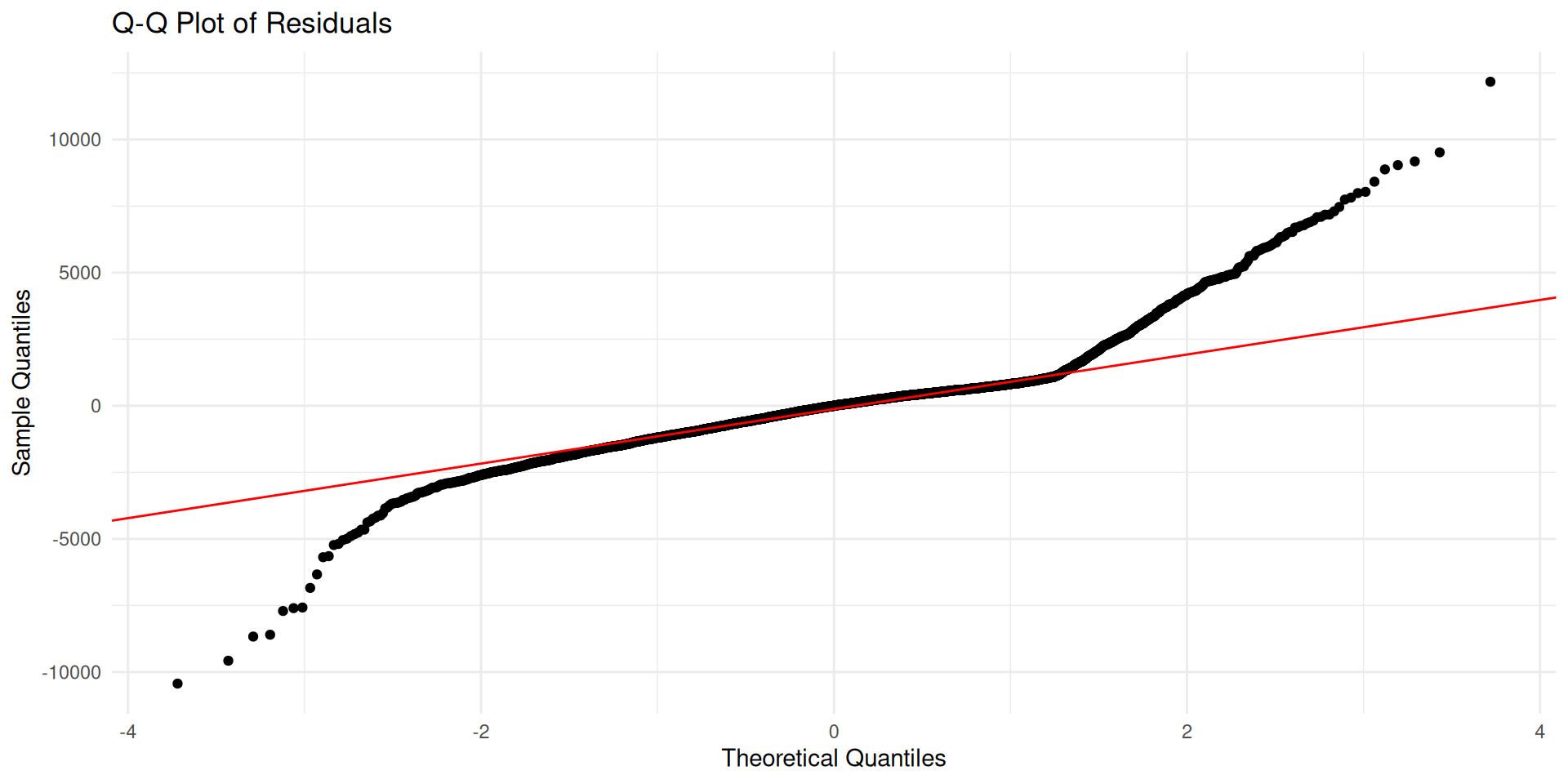
    • The Q-Q plot compares the quantiles of some sample to the theoretical quantiles from a pre-specified distribution (such as the normal distribution)

Histogram of residuals

Q-Q plot of residuals

New geom_*() unlocked!

ggplot(diamonds_aug, aes(sample = .resid)) +
  stat_qq(size = 1.5) +
  stat_qq_line(color = "red") +
  labs(
    title = "Q-Q Plot of Residuals",
    x = "Theoretical Quantiles",
    y = "Sample Quantiles"
  ) +
  theme_minimal()

Again, what are we looking for?

  • Normality: We expect to see normally distributed residuals, centered at 0. In the Q-Q plot, we would expect to see minimal deviation from the reference line

  • Note that in the Q-Q plot, it’s ok if we see “some degree” of deviation (especially in the tails), but if there is a clear pattern or many observations which appear to be “off,” then that’s a clue that normality might be violated

Based on the histogram and Q-Q plot, what do you think of the normality assumption underlying our simple linear regression model predicting diamond price from carat?

From SLR to MLR

  • We fit a simple linear regression model with only one predictor (y = price, x = carat)

  • However, these same sort of model assumption diagnostics that we saw (fitted vs. residuals plots, histograms of residuals, Q-Q plots) also apply to the multiple linear regression setting, since the residuals themselves are a function of all of the predictors

Takeaways

  • Linear regression relies on several assumptions about the relationship(s) between predictors, outcomes, and residuals

  • When these assumptions are reasonably satisfied, the estimated regression coefficients have desirable statistical properties, and the conclusions from our model are more trustworthy

  • Diagnostic plots help us assess whether the assumptions appear reasonable for our data

  • No dataset is perfect; small departures from assumptions are common and do not automatically invalidate a regression analysis

  • However, substantial violations should be acknowledged (discussion of limitations) and may motivate alternative modeling approaches or transformations

Looking Ahead

  • As budding statistical analysts, it is our responsibility to evaluate these assumptions rather than simply fit a model and report the results

  • If you choose the “statistical modeling” project path, one component of your final report must be an assessment of these linear regression assumptions for your final regression model